AWS VS OpenStack?????

Let us compare the popularity of two top cloud-computing platforms:
1) the infamous Amazon Web Services, which companies typically leverage for the speed and convenience of Amazon's global, hosted, cloud-computing infrastructure, and
2) the increasingly versatile OpenStack, which allows organizations to roll their own cloud-computing services on standard hardware.

OpenStack has similarly grown in popularity since its launch in 2010, having had a nice jump in the Spring of 2013. Some of the more notable companies contributing to OpenStack include: AT&T, MD, Canonical, Cisco, Citrix, Comcast, Cray, Dell, Dreamhost, EMC, Ericsson, Fujitsu, GoDaddy, Google, HP, Hitachi, Huawei, IBM, Intel, Juniper Networks, Mirantis, Oracle, Red Hat, SUSE Linux, VMware, and Yahoo!.
While OpenStack has a lot of diverse contributors, AWS is the fifth largest web hosting provider globally.
Worldwide Market Share by Number of Clients in 2015:

1. GoDaddy - 4.26%
2. BlueHost - 2.56%
3. Host Gator - 2.15%
4. OVH.com - 1.91%
5. Amazon Web Services - 1.81%
6. Rackspace - 1.59%
7. 1&1 - 1.54%
8. Hetzner - 1.29%
9. SoftLayer - 1.19%
10. DreamHost - 1.01%

source: http://hostadvice.com/marketshare/ (2015)

As an open-source cloud-computing protocol, OpenStack obviously can't compete on these terms with a multi-billion dollar cloud-computing and software-as-a-service company. There are a number selling points to consider, however:

• WalMart uses OpenStack to coordinate 100,000+ cores, this provided 100% uptime during Black Friday last year
• Developers gave over 300 talks at the OpenStack Summit in Tokyo this October
• Debian, Canonical, Red Hat, and SUSE Linux all support OpenStack and are active contributors
• OpenStack has enabled companies like Disney, Bloomberg, and Wells Fargo to manage their own clouds at a fraction of the cost of proprietary solutions like AWS
• OpenStack is the only solution that supports mixed hypervisor and bare metal server environments

I think these points lend themselves to the conclusion that adoption and further development in OpenStack are likely to keep pace.

Here is a subset of AWS services:

In the Compute realm we have...

• Amazon Elastic Compute Cloud (EC2) scalable virtual private servers using Xen
• Amazon Elastic MapReduce (EMR) Hadoop-based big data analytics

In Networking we have...

• Amazon Route 53 scalable DNS
• Amazon Virtual Private Cloud (VPC) isolated EC2 instances with the ability to extend corporate networks VPN
• Amazon Elastic Load Balancing (ELB)

In Content Delivery we have...

• Amazon CloudFront CDN

In Storage we have...

• Amazon Simple Storage Service (S3)
• Amazon Glacier low-cost, long-term storage for data archival
• Amazon Elastic File System (EFS) to accompany EC2

In the Database realm we have...

• Amazon DynamoDB low-latency NoSQL SSD-backed databases
• Amazon Relational Database Service (RDS) with MySQL, Oracle, SQL Server, and PostgreSQL support
• Amazon SimpleDB distributed database with EC2 and S3 interoperability, written in Erlang

In the Deployment realm we have...

• AWS Elastic Beanstalk for quick deployment and cloud app management
• AWS OpsWorks EC2 configuration services via Chef, which we discussed previously

In Management we have...

• Amazon Identity and Access Management (IAM) to authenticate into the various services
• AWS Directory Service for tying into an on-premises Microsoft Active Directory or for setting up a new stand-alone AWS directory
• Amazon CloudWatch for application and resource monitoring
• Amazon CloudHSM Hardware Security Module for data security and for meeting regulatory compliance requirements
• AWS Key Management Service (KMS) for creating and managing encryption keys

In the Application Services realm we have...

• Amazon DevPay (beta) for billing and account management
• Amazon Elastic Transcoder (ETS) for mobile video transcription from S3
• Amazon Simple Email Service (SES) for sending bulk and transactional email
• Amazon Simple Notification Service (SNS) multi-protocol application "push" notifications
• Amazon Cognito secure application-user data management and synchronization tool

In Analytics we have...

• Amazon Machine Learning for building regression models from publicly-available datasets

Here are the main components of the modular OpenStack architecture:

Compute (Nova)

• An Infrastructure as a Service (IaaS) system
• Management and automatation of pools of computer resources
• Bare metal and high-performance computing (HPC) configurations
• KVM, VMware, and Xen hypervisor virtualization
• Hyper-V and LXC containerization
• Python-based with various external libraries: Eventlet for concurrent programming, Kombu for AMQP communication, SQLAlchemy for database access, etc.
• Designed to scale horizontally on standard hardware with no proprietary hardware or software requirements
• Interoperable with legacy systems

Image Service (Glance)

• OpenStack Image Service for discovery, registration, and delivery of services for disk and server images
• Template-building from stored images
• Storage and cataloging of unlimited backups
• REST interface for querying disk image information
• Streaming of images to servers
• VMware integration, with vMotion Dynamic Resource Scheduling (DRS) and live migration of running virtual machines
• All OpenStack OS images built on virtual machines
• Maintenance of image metadata
• Creation, deletion, sharing, and duplification of images

Object Storage (Swift)

• Scalable redundant storage system
• Automatic replication of content from failed disks to other active nodes
• Suitable for inexpensive commodity hard drives and servers

Dashboard (Horizon)

• GUI for access, provision, and automation of cloud-based resources for administrators and users
• Third-party billing, monitoring, management tool integration
• Customizable (brandable) dashboard
• EC2 compatibility

Identity Service (Keystone)

• Unified authentication system across the cloud OS
• Integration with existing backend directory services such as LDAP
• Various authentication methods: username/password, token-based systems, and AWS-style logins
• Queryable, single registry of all deployed services, with programmatic determination of access for users and third-party tools

Networking (Neutron)

• Manual and automatic management of networks and IP addresses
• Distict networking models for different applications and user groups
• Flat networks (VLAN's) for separating servers and traffic.
• Static IP addresses, DHCP
• Floating IP addresses for dynamic rerouting to resources on the network
• Software-defined networking (SDN), OpenFlow, for multi-tenancy and scalability.
• Management of intrusion detection systems (IDS), load balancing, firewalls, VPN's, etc.

Block Storage (Cinder)

• Persistent block-level storage for databases and expandable file systems
• Block storage integration into OpenStack Compute and Dashboard for allocation of storage
• Various storage platforms supported: Ceph, CloudByte, Coraid, EMC (ScaleIO, VMAX and VNX), GlusterFS, Hitachi Data Systems, IBM Storage (Storwize family, SAN Volume Controller, XIV Storage System, and GPFS), Linux LIO, NetApp, Nexenta, Scality, SolidFire, HP (StoreVirtual and 3PAR StoreServ families) and Pure Storag
• Snapshot management for backing up data stored on block storage volumes
• Restoring of snapshots, use of snapshots as templates for new block storage volumes

Orchestration (Heat)

• Orchestratation of multiple composite cloud applications using templates
• OpenStack-native REST API
• CloudFormation-compatible Query API

Telemetry (Ceilometer)

• Billing system Single Point Of Contact
• Traceable, auditable delivery of counters for billing
• Counters extensible to new projects
• Independent data collection

Database (Trove)

• Database-as-a-service (DaaS) provisioning relational database engine
• DaaS non-relational database engine

Elastic Map Reduce (Sahara)

• Hadoop cluster provisioning
• Setting of parameters based on: Hadoop version, cluster topology, node hardware details, etc.
• Cluster deployment in minutes
• Scaling of already-provisioned clusters by adding and removing worker nodes on demand

Bare Metal Provisioning (Ironic)

• Provisioning of bare metal machines (as opposed to virtual machines)
• Bare-metal hypervisor API
• Plugins for interacting with bare-metal hypervisors
• PXE and IPMI simultaneous provisioning, turning machines on and off as needed
• Extensible with vendor-specific plugins for additional functionality

Multiple Tenant Cloud Messaging (Zaqar)

• Multi-tenant cloud messaging service for Web developers
• Some components inspired by Amazon's SQS, with additional semantics for event broadcasting
• Fully RESTful API for sending messages between various components of their SaaS and mobile applications
• Surfacing of events to end users and guest agents that run in the "over-cloud" layer

Shared File System Service (Manila)

• Vendor-agnostic share management API
• Create, delete, give/deny access to a share
• Support for commercial storage appliances from: EMC, NetApp, HP, IBM, Oracle, Quobyte, and Hitachi Data Systems
• Support for Red Hat's GlusterFS filesystem

DNSaaS (Designate)

• DNS as a Service

Security API (Barbican)

• REST API for secure storage, provisioning and management of secrets
• Built for use in all environments, including large ephemeral clouds

AWS Compatibility

• Interoperability with Amazon EC2 and Amazon S3
• Minimal effort to port AWS client applications to OpenStack

Multi tenancy: AWS vs OpenStack

The first conceptual difference between AWS and OpenStack is about multi-tenancy. OpenStack offers a multi-layer tenant mechanism with domain and projects. A domain is a collection of users, groups, and projects, in a way parallel to AWS’s account. LDAP groups are attached to domains. OpenStack’s Project is a container of virtual resources such as virtual machines, networks and volumes. Using projects, users can establish several isolated and independently controlled groups of resources that serve different objectives. In the Kilo release, Keystone introduced the hierarchical multi-tenancy concept, using sub-projects.
Accommodating more than one million customers, Amazon Web Services is a multi-tenant cloud by nature; however, at the account level, a single user receives a single tenant experience. Having said that, AWS offers Virtual Private Cloud, VPC, which is somewhat parallel to OpenStack’s project. Amazon’s VPC lets the user provision a logically isolated section of the Amazon Web Services (AWS) cloud where the user can launch AWS resources in a virtual network that s/he defines.  AWS’s VPC is limited to one router and one IP block; though not compulsory, this is a common practice for OpenStack projects. It is worth noting that all EC2’s virtual networking capabilities are only available using VPC.
On the other hand, unlike OpenStack, Amazon’s VPC offers extremely valuable tools that simplify the establishment of secured connectivity between VPCs and between VPC and on-premise resources. The classical use case for enterprises is running the web servers or the entire customer facing application on Amazon’s public cloud, while keeping the rest of the servers on-premise. Through its API, Amazon allows the user to establish a VPN connection and even control the customer’s and AWS’s gateways. This is extremely valuable for enterprises that chose the hybrid cloud path, especially given the fact that Amazon has integrated its VPN gateway with the market leading VPN CPEs (customer premise equipment). OpenStack’s Neutron project does offers VPN as a Service capabilities (VPNaaS); however, it is experimental and lacks the end-to-end integration that Amazon provides.

Networking: Neutron vs AWS VPC

From the network perspective, while OpenStack provides control over the L2 elements of the virtual network, AWS exposes only subnets. OpenStack Neutron’s API allows granular control of elements such as ports (the connection point for attaching a virtual server to a virtual network) and the ability to allocate VLAN IDs that correspond to VLANs present in the physical network. This is especially useful for provider networks, which are mapped to existing physical networks in the data center. Those differences are again attributed to the different concepts of AWS and OpenStack. In the private cloud, the user manages the physical networking by himself. Thus, it is crucial for virtual networking to be fully integrated with the physical data center networking. However, the public cloud is a managed service that takes all the hassle of physical network management away from the user, therefore  providing control on L2 is irrelevant to the user.
As for Layer 3 networking, conceptually, Amazon’s AWS and OpenStack’s Neutron provides comparable capabilities. Both cloud services allow creation of network subnets. OpenStack allows use of several subnets on the same virtual network, although it is not a common practice. AWS allows users to define Elastic IP addresses, which are public IP addresses reachable from the Internet. OpenStack offers a similar mechanism, the floating IP, which is part of the virtual router’s API.
Both clouds provide routing services; in AWS each VPC includes an implicit virtual router and the API allows the user to set the routing table (which contains a set of rules, called routes, that are used to determine where network traffic is directed). OpenStack’s Neutron API also allows management of the routing table;  however, it also allows management of the router entities themselves and does not limiting the number of routers per project. Moreover, a single router can be connected to more than one project.
From a network security perspective, AWS and OpenStack offer similar mechanisms. Security groups are used to inspect the traffic at the instance level. Networking ACLs and virtual firewalls are used by AWS and OpenStack respectively to inspect traffic going between subnets. There are minor nuances unique to each API; however, the general concept is very similar.

Here we compare some main components of AWS and OpenStack

Compute

 Why you need it?

To run an application you need a server with CPU, memory and storage, with or without pre-installed operating systems and applications.

	OpenStack	AWS
Definition Compute is virtual machines/servers	Instance	Instance/VM
Sizes How much memory and CPU and temporary (ephemeral) storage is assigned to the instances/VM.	Flavors: Variety of sizes: micro, small, medium, large etc.	Variety of sizes: micro, small, medium, large etc.
Operating systems offered What operating systems does the cloud offer to end-users	Whatever operating systems the cloud administrators host on the OpenStack cloud. (Red Hat certifies Microsoft Windows, RHEL and SUSE)	AMIs provided by the AWS marketplace.
Templates/images A base configuration of a virtual machine, from which other virtual machines can be created. Catalogs of virtual machine images can be created from which users can select a virtual machine.	Glance  OpenStack administrators upload images and create catalogs for users. Users can upload their own images.	(AMI) Amazon Machine Image AWS provides an online marketplace of pre-defined images. Users can upload their own images.

Networking

 Why you need it?

To network virtual servers to each other. You also need to control who can access the server. You want to protect/firewall the server especially if it is exposed to the Internet.

	OpenStack	AWS
Definition Networking provides connectivity for users to virtual machines. Connects virtual machines to one another and to external networks (the Internet).	Neutron	Networking
A private IP address internal only and non-routable to the Internet	Every virtual instance is automatically assigned a private IP address, typically using DHCP.	AWS allocates a private IP address for the instance using DHCP.
Public IP address	A floating IP is a public IP address, that you can dynamically add to a running virtual instance.	AWS public IP address is mapped to the primary private IP address.
Networking service	You can create networks and networking functions, eg. L3 forwarding, NAT, edge firewalls, and IPsec VPN.	Virtual routers or switches can be added if you use AWS VPC, a virtual public cloud.
Load Balance VM traffic	OpenStack LBaaS (Load Balancing as a Service) balances traffic from one network to application services.	ELB (Elastic Load Balancing) automatically distributes incoming application traffic across Amazon EC2 instances.
DNS. Manage the DNS entries for your virtual servers and web applications.	The OpenStack DNS project (Designate) is in “incubation” and is not part of core OpenStack (as of the April 2015 Kilo release).	Route 53 –  AWS’s DNS service.
SRIOV A method of device virtualization that provides higher I/O performance and lower CPU utilization compared to traditional implementations.	Each SR-IOV port is associated with a virtual function (VF). SR-IOV ports may be provided by Hardware-based Virtual Ethernet Bridging or they may be extended to an upstream physical switch (IEEE 802.1br).	AWS support enhanced networking capabilities using SR-IOV, provides higher packet per second (PPS) performance, lower inter-instance latencies, and very low network jitter.

Monitoring

Why you need it?

You get insight into usage patterns and utilization of the physical and virtual resources. You may want to account for individual usage and optionally bill users for their usage.

	OpenStack	AWS
Definition Monitoring provides metering and usage of the cloud.	Ceilometer	Cloudwatch
System-wide metering and usage. Option to bill users for their usage	To collect measurements of the utilization of the physical and virtual resources comprising deployed clouds. Persist data for subsequent retrieval and analysis, and trigger actions when defined criteria are met.	Monitoring service for AWS cloud resources and the applications  on AWS. Collect and track metrics, collect and monitor log files, and set alarms.

Security

Why you need it?

You need the  option of public key cryptography for SSH and password decryption. You want to firewall virtual machines to only allow certain traffic in (ingress) or out (egress).

	OpenStack	AWS
Definition Control access to your virtual machines.	Keypairs, security groups.	Keypairs, security groups.
Key pairs To login to your VM or instance, you must create a key pair. Linux: used to SSH. Windows: used to decrypt the Administrator password.	When you launch a virtual machine, you can inject a key pair, which provides SSH access to your instance.	To log in to your instance, specify the name of the key pair when you launch the instance, and provide the private key when you connect to the instance.
Assign and control access to VM instances. A security group is a named collection of network access rules that limit the traffic that access an instance. When you launch an instance, you can assign one or more security groups to it.	Supported	Supported

Read More

Intro to Redis

Introduction to Redis

Redis is an open source (BSD licensed), in-memory data structure store, used as a database, cache and message broker. It supports data structures such as strings, hashes, lists, sets, sorted sets with range queries, bitmaps, hyperlog logs and geospatial indexes with radius queries. Redis has built-in replication, Lua scripting, LRU eviction, transactions and different levels of on-disk persistence, and provides high availability via Redis Sentinel and automatic partitioning with Redis Cluster.

You can run atomic operations on these types, like appending to a string; incrementing the value in a hash; pushing an element to a list; computing set intersection, union and difference; or getting the member with highest ranking in a sorted set.

In order to achieve its outstanding performance, Redis works with an in-memory data set. Depending on your use case, you can persist it either by dumping the data set to disk every once in a while, or by appending each command to a log. Persistence can be optionally disabled, if you just need a feature-rich, networked, in-memory cache.

Redis also supports trivial-to-setup master-slave asynchronous replication, with very fast non-blocking first synchronization, auto-re-connection with partial re-synchronization on net split.

Other features include:

•     Transactions
•     Pub/Sub
•     Lua scripting
•     Keys with a limited time-to-live
•     LRU eviction of keys
•     Automatic fail over

You can use Redis from most programming languages out there.

Redis is written in ANSI C and works in most POSIX systems like Linux, *BSD, OS X without external dependencies. Linux and OS X are the two operating systems where Redis is developed and more tested, and we recommend using Linux for deploying. Redis may work in Solaris-derived systems like SmartOS, but the support is best effort. There is no official support for Windows builds, but Microsoft develops and maintains a Win-64 port of Redis.

An introduction to Redis data types and abstractions

Redis is not a plain key-value store, it is actually a data structures server, supporting different kinds of values. What this means is that, while in traditional key-value stores you associated string keys to string values, in Redis the value is not limited to a simple string, but can also hold more complex data structures. The following is the list of all the data structures supported by Redis, which will be covered separately in this tutorial:

• Binary-safe strings.
• Lists: collections of string elements sorted according to the order of insertion. They are basically linked lists.
• Sets: collections of unique, unsorted string elements.
• Sorted sets, similar to Sets but where every string element is associated to a floating number value, called score. The elements are always taken sorted by their score, so unlike Sets it is possible to retrieve a range of elements (for example you may ask: give me the top 10, or the bottom 10).
• Hashes, which are maps composed of fields associated with values. Both the field and the value are strings. This is very similar to Ruby or Python hashes.
• Bit arrays (or simply bitmaps): it is possible, using special commands, to handle String values like an array of bits: you can set and clear individual bits, count all the bits set to 1, find the first set or unset bit, and so forth.
• HyperLogLogs: this is a probabilistic data structure which is used in order to estimate the cardinality of a set. Don't be scared, it is simpler than it seems... See later in the HyperLogLog section of this tutorial.

It's not always trivial to grasp how these data types work and what to use in order to solve a given problem from the command reference, so this document is a crash course to Redis data types and their most common patterns.
For all the examples we'll use the redis-cli utility, a simple but handy command-line utility, to issue commands against the Redis server.

Redis keys

Redis keys are binary safe, this means that you can use any binary sequence as a key, from a string like "foo" to the content of a JPEG file. The empty string is also a valid key.
A few other rules about keys:

• Very long keys are not a good idea. For instance a key of 1024 bytes is a bad idea not only memory-wise, but also because the lookup of the key in the dataset may require several costly key-comparisons. Even when the task at hand is to match the existence of a large value, hashing it (for example with SHA1) is a better idea, especially from the perspective of memory and bandwidth.
• Very short keys are often not a good idea. There is little point in writing "u1000flw" as a key if you can instead write "user:1000:followers". The latter is more readable and the added space is minor compared to the space used by the key object itself and the value object. While short keys will obviously consume a bit less memory, your job is to find the right balance.
• Try to stick with a schema. For instance "object-type:id" is a good idea, as in "user:1000". Dots or dashes are often used for multi-word fields, as in "comment:1234:reply.to" or "comment:1234:reply-to".
• The maximum allowed key size is 512 MB.

Redis Strings

The Redis String type is the simplest type of value you can associate with a Redis key. It is the only data type in Memcached, so it is also very natural for newcomers to use it in Redis.
Since Redis keys are strings, when we use the string type as a value too, we are mapping a string to another string. The string data type is useful for a number of use cases, like caching HTML fragments or pages.
Let's play a bit with the string type, using redis-cli (all the examples will be performed via redis-cli in this tutorial).

> set mykey somevalue
OK
> get mykey
"somevalue"

As you can see using the SET and the GET commands are the way we set and retrieve a string value. Note that SET will replace any existing value already stored into the key, in the case that the key already exists, even if the key is associated with a non-string value. So SET performs an assignment.
Values can be strings (including binary data) of every kind, for instance you can store a jpeg image inside a key. A value can't be bigger than 512 MB.
The SET command has interesting options, that are provided as additional arguments. For example, I may ask SET to fail if the key already exists, or the opposite, that it only succeed if the key already exists:

> set mykey newval nx
(nil)
> set mykey newval xx
OK

Even if strings are the basic values of Redis, there are interesting operations you can perform with them. For instance, one is atomic increment:

> set counter 100
OK
> incr counter
(integer) 101
> incr counter
(integer) 102
> incrby counter 50
(integer) 152

The INCR command parses the string value as an integer, increments it by one, and finally sets the obtained value as the new value. There are other similar commands like INCRBY, DECR and DECRBY. Internally it's always the same command, acting in a slightly different way.
What does it mean that INCR is atomic? That even multiple clients issuing INCR against the same key will never enter into a race condition. For instance, it will never happen that client 1 reads "10", client 2 reads "10" at the same time, both increment to 11, and set the new value to 11. The final value will always be 12 and the read-increment-set operation is performed while all the other clients are not executing a command at the same time.
There are a number of commands for operating on strings. For example the GETSET command sets a key to a new value, returning the old value as the result. You can use this command, for example, if you have a system that increments a Redis key using INCR every time your web site receives a new visitor. You may want to collect this information once every hour, without losing a single increment. You can GETSET the key, assigning it the new value of "0" and reading the old value back.
The ability to set or retrieve the value of multiple keys in a single command is also useful for reduced latency. For this reason there are the MSET and MGET commands:

> mset a 10 b 20 c 30
OK
> mget a b c
1) "10"
2) "20"
3) "30"

When MGET is used, Redis returns an array of values.

Altering and querying the key space

There are commands that are not defined on particular types, but are useful in order to interact with the space of keys, and thus, can be used with keys of any type.
For example the EXISTS command returns 1 or 0 to signal if a given key exists or not in the database, while the DEL command deletes a key and associated value, whatever the value is.

> set mykey hello
OK
> exists mykey
(integer) 1
> del mykey
(integer) 1
> exists mykey
(integer) 0

From the examples you can also see how DEL itself returns 1 or 0 depending on whether the key was removed (it existed) or not (there was no such key with that name).
There are many key space related commands, but the above two are the essential ones together with the TYPE command, which returns the kind of value stored at the specified key:

> set mykey x
OK
> type mykey
string
> del mykey
(integer) 1
> type mykey
none

Redis expires: keys with limited time to live

Before continuing with more complex data structures, we need to discuss another feature which works regardless of the value type, and is called Redis expires. Basically you can set a timeout for a key, which is a limited time to live. When the time to live elapses, the key is automatically destroyed, exactly as if the user called the DEL command with the key.
A few quick info about Redis expires:

• They can be set both using seconds or milliseconds precision.
• However the expire time resolution is always 1 millisecond.
• Information about expires are replicated and persisted on disk, the time virtually passes when your Redis server remains stopped (this means that Redis saves the date at which a key will expire).

Setting an expire is trivial:

> set key some-value
OK
> expire key 5
(integer) 1
> get key (immediately)
"some-value"
> get key (after some time)
(nil)

The key vanished between the two GET calls, since the second call was delayed more than 5 seconds. In the example above we used EXPIRE in order to set the expire (it can also be used in order to set a different expire to a key already having one, like PERSIST can be used in order to remove the expire and make the key persistent forever). However we can also create keys with expires using other Redis commands. For example using SET options:

> set key 100 ex 10
OK
> ttl key
(integer) 9

The example above sets a key with the string value 100, having an expire of ten seconds. Later the TTL command is called in order to check the remaining time to live for the key.
In order to set and check expires in milliseconds, check the PEXPIRE and the PTTL commands, and the full list of SET options.

Redis Lists

To explain the List data type it's better to start with a little bit of theory, as the term List is often used in an improper way by information technology folks. For instance "Python Lists" are not what the name may suggest (Linked Lists), but rather Arrays (the same data type is called Array in Ruby actually).
From a very general point of view a List is just a sequence of ordered elements: 10,20,1,2,3 is a list. But the properties of a List implemented using an Array are very different from the properties of a List implemented using a Linked List.
Redis lists are implemented via Linked Lists. This means that even if you have millions of elements inside a list, the operation of adding a new element in the head or in the tail of the list is performed in constant time. The speed of adding a new element with the LPUSH command to the head of a list with ten elements is the same as adding an element to the head of list with 10 million elements.
What's the downside? Accessing an element by index is very fast in lists implemented with an Array (constant time indexed access) and not so fast in lists implemented by linked lists (where the operation requires an amount of work proportional to the index of the accessed element).
Redis Lists are implemented with linked lists because for a database system it is crucial to be able to add elements to a very long list in a very fast way. Another strong advantage, as you'll see in a moment, is that Redis Lists can be taken at constant length in constant time.
When fast access to the middle of a large collection of elements is important, there is a different data structure that can be used, called sorted sets. Sorted sets will be covered later in this tutorial.

First steps with Redis Lists

The LPUSH command adds a new element into a list, on the left (at the head), while the RPUSH command adds a new element into a list ,on the right (at the tail). Finally the LRANGE command extracts ranges of elements from lists:

> rpush mylist A
(integer) 1
> rpush mylist B
(integer) 2
> lpush mylist first
(integer) 3
> lrange mylist 0 -1
1) "first"
2) "A"
3) "B"

Note that LRANGE takes two indexes, the first and the last element of the range to return. Both the indexes can be negative, telling Redis to start counting from the end: so -1 is the last element, -2 is the penultimate element of the list, and so forth.
As you can see RPUSH appended the elements on the right of the list, while the final LPUSH appended the element on the left.
Both commands are variadic commands, meaning that you are free to push multiple elements into a list in a single call:

> rpush mylist 1 2 3 4 5 "foo bar"
(integer) 9
> lrange mylist 0 -1
1) "first"
2) "A"
3) "B"
4) "1"
5) "2"
6) "3"
7) "4"
8) "5"
9) "foo bar"

An important operation defined on Redis lists is the ability to pop elements. Popping elements is the operation of both retrieving the element from the list, and eliminating it from the list, at the same time. You can pop elements from left and right, similarly to how you can push elements in both sides of the list:

> rpush mylist a b c
(integer) 3
> rpop mylist
"c"
> rpop mylist
"b"
> rpop mylist
"a"

We added three elements and popped three elements, so at the end of this sequence of commands the list is empty and there are no more elements to pop. If we try to pop yet another element, this is the result we get:

> rpop mylist
(nil)

Redis returned a NULL value to signal that there are no elements into the list.

Common use cases for lists

Lists are useful for a number of tasks, two very representative use cases are the following:

• Remember the latest updates posted by users into a social network.
• Communication between processes, using a consumer-producer pattern where the producer pushes items into a list, and a consumer (usually a worker) consumes those items and executed actions. Redis has special list commands to make this use case both more reliable and efficient.

For example both the popular Ruby libraries resque and sidekiq use Redis lists under the hood in order to implement background jobs.
The popular Twitter social network takes the latest tweets posted by users into Redis lists.
To describe a common use case step by step, imagine your home page shows the latest photos published in a photo sharing social network and you want to speedup access.

• Every time a user posts a new photo, we add its ID into a list with LPUSH.
• When users visit the home page, we use LRANGE 0 9 in order to get the latest 10 posted items.

Capped lists

In many use cases we just want to use lists to store the latest items, whatever they are: social network updates, logs, or anything else.
Redis allows us to use lists as a capped collection, only remembering the latest N items and discarding all the oldest items using the LTRIM command.
The LTRIM command is similar to LRANGE, but instead of displaying the specified range of elements it sets this range as the new list value. All the elements outside the given range are removed.
An example will make it more clear:

> rpush mylist 1 2 3 4 5
(integer) 5
> ltrim mylist 0 2
OK
> lrange mylist 0 -1
1) "1"
2) "2"
3) "3"

The above LTRIM command tells Redis to take just list elements from index 0 to 2, everything else will be discarded. This allows for a very simple but useful pattern: doing a List push operation + a List trim operation together in order to add a new element and discard elements exceeding a limit:

LPUSH mylist 
LTRIM mylist 0 999

The above combination adds a new element and takes only the 1000 newest elements into the list. With LRANGE you can access the top items without any need to remember very old data.

Note: while LRANGE is technically an O(N) command, accessing small ranges towards the head or the tail of the list is a constant time operation.

Automatic creation and removal of keys

So far in our examples we never had to create empty lists before pushing elements, or removing empty lists when they no longer have elements inside. It is Redis' responsibility to delete keys when lists are left empty, or to create an empty list if the key does not exist and we are trying to add elements to it, for example, with LPUSH.
This is not specific to lists, it applies to all the Redis data types composed of multiple elements -- Sets, Sorted Sets and Hashes.
Basically we can summarize the behavior with three rules:

1. When we add an element to an aggregate data type, if the target key does not exist, an empty aggregate data type is created before adding the element.
2. When we remove elements from an aggregate data type, if the value remains empty, the key is automatically destroyed.
3. Calling a read-only command such as LLEN (which returns the length of the list), or a write command removing elements, with an empty key, always produces the same result as if the key is holding an empty aggregate type of the type the command expects to find.

Examples of rule 1:

> del mylist
(integer) 1
> lpush mylist 1 2 3
(integer) 3

However we can't perform operations against the wrong type if the key exists:

> set foo bar
OK
> lpush foo 1 2 3
(error) WRONGTYPE Operation against a key holding the wrong kind of value
> type foo
string

Example of rule 2:

> lpush mylist 1 2 3
(integer) 3
> exists mylist
(integer) 1
> lpop mylist
"3"
> lpop mylist
"2"
> lpop mylist
"1"
> exists mylist
(integer) 0

The key no longer exists after all the elements are popped.
Example of rule 3:

> del mylist
(integer) 0
> llen mylist
(integer) 0
> lpop mylist
(nil)

Redis Hashes

Redis hashes look exactly how one might expect a "hash" to look, with field-value pairs:

> hmset user:1000 username antirez birthyear 1977 verified 1
OK
> hget user:1000 username
"antirez"
> hget user:1000 birthyear
"1977"
> hgetall user:1000
1) "username"
2) "antirez"
3) "birthyear"
4) "1977"
5) "verified"
6) "1"

While hashes are handy to represent objects, actually the number of fields you can put inside a hash has no practical limits (other than available memory), so you can use hashes in many different ways inside your application.
The command HMSET sets multiple fields of the hash, while HGET retrieves a single field. HMGET is similar to HGET but returns an array of values:

> hmget user:1000 username birthyear no-such-field
1) "antirez"
2) "1977"
3) (nil)

There are commands that are able to perform operations on individual fields as well, like HINCRBY:

> hincrby user:1000 birthyear 10
(integer) 1987
> hincrby user:1000 birthyear 10
(integer) 1997

You can find the full list of hash commands in the documentation.
It is worth noting that small hashes (i.e., a few elements with small values) are encoded in special way in memory that make them very memory efficient.

Redis Sets

Redis Sets are unordered collections of strings. The SADD command adds new elements to a set. It's also possible to do a number of other operations against sets like testing if a given element already exists, performing the intersection, union or difference between multiple sets, and so forth.

> sadd myset 1 2 3
(integer) 3
> smembers myset
1. 3
2. 1
3. 2

Here I've added three elements to my set and told Redis to return all the elements. As you can see they are not sorted -- Redis is free to return the elements in any order at every call, since there is no contract with the user about element ordering.
Redis has commands to test for membership. For example, checking if an element exists:

> sismember myset 3
(integer) 1
> sismember myset 30
(integer) 0

"3" is a member of the set, while "30" is not.
Sets are good for expressing relations between objects. For instance we can easily use sets in order to implement tags.
A simple way to model this problem is to have a set for every object we want to tag. The set contains the IDs of the tags associated with the object.
One illustration is tagging news articles. If article ID 1000 is tagged with tags 1, 2, 5 and 77, a set can associate these tag IDs with the news item:

> sadd news:1000:tags 1 2 5 77
(integer) 4

We may also want to have the inverse relation as well: the list of all the news tagged with a given tag:

> sadd tag:1:news 1000
(integer) 1
> sadd tag:2:news 1000
(integer) 1
> sadd tag:5:news 1000
(integer) 1
> sadd tag:77:news 1000
(integer) 1

To get all the tags for a given object is trivial:

> smembers news:1000:tags
1. 5
2. 1
3. 77
4. 2

Note: in the example we assume you have another data structure, for example a Redis hash, which maps tag IDs to tag names.
There are other non trivial operations that are still easy to implement using the right Redis commands. For instance we may want a list of all the objects with the tags 1, 2, 10, and 27 together. We can do this using the SINTER command, which performs the intersection between different sets. We can use:

> sinter tag:1:news tag:2:news tag:10:news tag:27:news
... results here ...

In addition to intersection you can also perform unions, difference, extract a random element, and so forth.
The command to extract an element is called SPOP, and is handy to model certain problems. For example in order to implement a web-based poker game, you may want to represent your deck with a set. Imagine we use a one-char prefix for (C)lubs, (D)iamonds, (H)earts, (S)pades:

>  sadd deck C1 C2 C3 C4 C5 C6 C7 C8 C9 C10 CJ CQ CK
   D1 D2 D3 D4 D5 D6 D7 D8 D9 D10 DJ DQ DK H1 H2 H3
   H4 H5 H6 H7 H8 H9 H10 HJ HQ HK S1 S2 S3 S4 S5 S6
   S7 S8 S9 S10 SJ SQ SK
   (integer) 52

Now we want to provide each player with 5 cards. The SPOP command removes a random element, returning it to the client, so it is the perfect operation in this case.
However if we call it against our deck directly, in the next play of the game we'll need to populate the deck of cards again, which may not be ideal. So to start, we can make a copy of the set stored in the deck key into the game:1:deck key.
This is accomplished using SUNIONSTORE, which normally performs the union between multiple sets, and stores the result into another set. However, since the union of a single set is itself, I can copy my deck with:

> sunionstore game:1:deck deck
(integer) 52

Now I'm ready to provide the first player with five cards:

> spop game:1:deck
"C6"
> spop game:1:deck
"CQ"
> spop game:1:deck
"D1"
> spop game:1:deck
"CJ"
> spop game:1:deck
"SJ"

One pair of jacks, not great...
This is a good time to introduce the set command that provides the number of elements inside a set. This is often called the cardinality of a set in the context of set theory, so the Redis command is called SCARD.

> scard game:1:deck
(integer) 47

The math works: 52 - 5 = 47.
When you need to just get random elements without removing them from the set, there is the SRANDMEMBER command suitable for the task. It also features the ability to return both repeating and non-repeating elements.

Redis Sorted sets

Sorted sets are a data type which is similar to a mix between a Set and a Hash. Like sets, sorted sets are composed of unique, non-repeating string elements, so in some sense a sorted set is a set as well.
However while elements inside sets are not ordered, every element in a sorted set is associated with a floating point value, called the score (this is why the type is also similar to a hash, since every element is mapped to a value).
Moreover, elements in a sorted sets are taken in order (so they are not ordered on request, order is a peculiarity of the data structure used to represent sorted sets). They are ordered according to the following rule:

• If A and B are two elements with a different score, then A > B if A.score is > B.score.
• If A and B have exactly the same score, then A > B if the A string is lexicographically greater than the B string. A and B strings can't be equal since sorted sets only have unique elements.

Let's start with a simple example, adding a few selected hackers names as sorted set elements, with their year of birth as "score".

> zadd hackers 1940 "Alan Kay"
(integer) 1
> zadd hackers 1957 "Sophie Wilson"
(integer) 1
> zadd hackers 1953 "Richard Stallman"
(integer) 1
> zadd hackers 1949 "Anita Borg"
(integer) 1
> zadd hackers 1965 "Yukihiro Matsumoto"
(integer) 1
> zadd hackers 1914 "Hedy Lamarr"
(integer) 1
> zadd hackers 1916 "Claude Shannon"
(integer) 1
> zadd hackers 1969 "Linus Torvalds"
(integer) 1
> zadd hackers 1912 "Alan Turing"
(integer) 1

As you can see ZADD is similar to SADD, but takes one additional argument (placed before the element to be added) which is the score. ZADD is also variadic, so you are free to specify multiple score-value pairs, even if this is not used in the example above.
With sorted sets it is trivial to return a list of hackers sorted by their birth year because actually they are already sorted.
Implementation note: Sorted sets are implemented via a dual-ported data structure containing both a skip list and a hash table, so every time we add an element Redis performs an O(log(N)) operation. That's good, but when we ask for sorted elements Redis does not have to do any work at all, it's already all sorted:

> zrange hackers 0 -1
1) "Alan Turing"
2) "Hedy Lamarr"
3) "Claude Shannon"
4) "Alan Kay"
5) "Anita Borg"
6) "Richard Stallman"
7) "Sophie Wilson"
8) "Yukihiro Matsumoto"
9) "Linus Torvalds"

Note: 0 and -1 means from element index 0 to the last element (-1 works here just as it does in the case of the LRANGE command).
What if I want to order them the opposite way, youngest to oldest? Use ZREVRANGE instead of ZRANGE:

> zrevrange hackers 0 -1
1) "Linus Torvalds"
2) "Yukihiro Matsumoto"
3) "Sophie Wilson"
4) "Richard Stallman"
5) "Anita Borg"
6) "Alan Kay"
7) "Claude Shannon"
8) "Hedy Lamarr"
9) "Alan Turing"

It is possible to return scores as well, using the WITHSCORES argument:

> zrange hackers 0 -1 withscores
1) "Alan Turing"
2) "1912"
3) "Hedy Lamarr"
4) "1914"
5) "Claude Shannon"
6) "1916"
7) "Alan Kay"
8) "1940"
9) "Anita Borg"
10) "1949"
11) "Richard Stallman"
12) "1953"
13) "Sophie Wilson"
14) "1957"
15) "Yukihiro Matsumoto"
16) "1965"
17) "Linus Torvalds"
18) "1969"

Read More

Intro to Kafka

Introduction

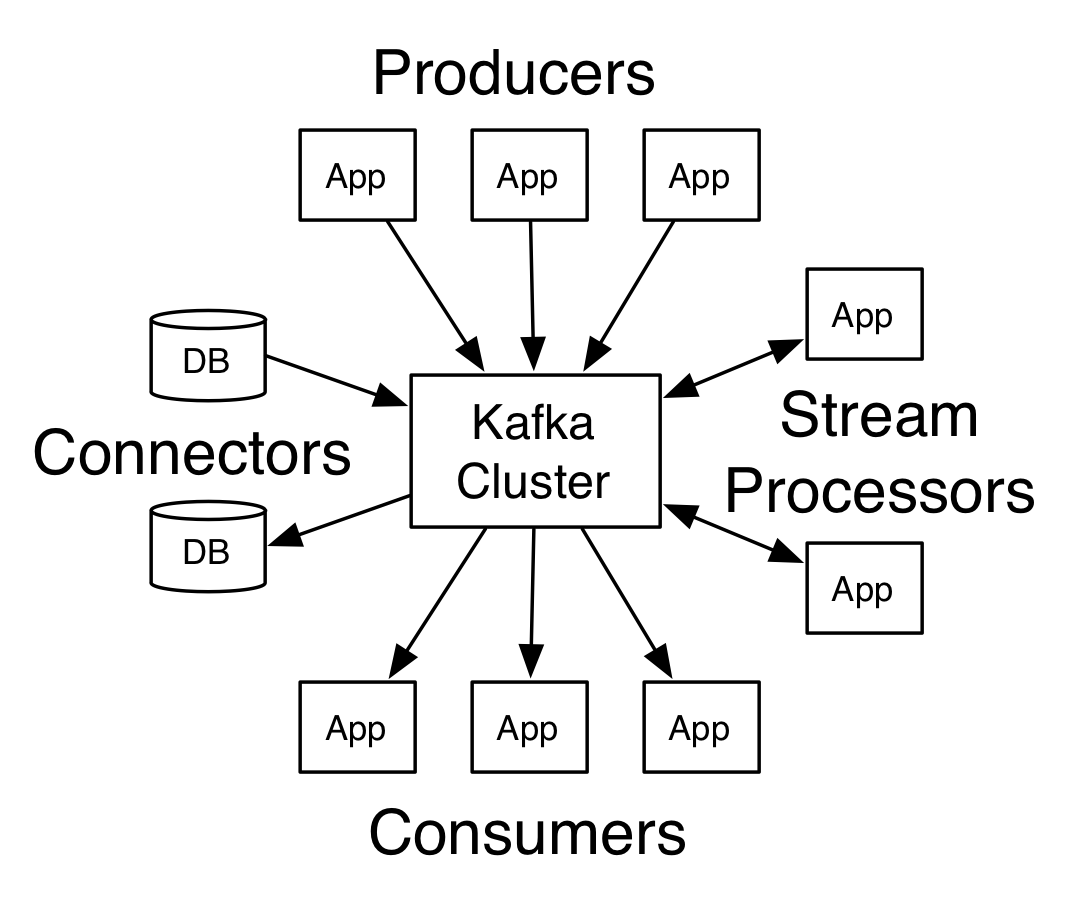
Apache Kafk is a distributed streaming platform. What exactly does that mean?

We think of a streaming platform as having three key capabilities:

1. It lets you publish and subscribe to streams of records. In this respect it is similar to a message queue or enterprise messaging system.
2. It lets you store streams of records in a fault-tolerant way.
3. It lets you process streams of records as they occur.

What is Kafka good for?
It gets used for two broad classes of application:

1. Building real-time streaming data pipelines that reliably get data between systems or applications
2. Building real-time streaming applications that transform or react to the streams of data

To understand how Kafka does these things, let's dive in and explore Kafka's capabilities from the bottom up.
First a few concepts:

• Kafka is run as a cluster on one or more servers.
• The Kafka cluster stores streams of records in categories called topics.
• Each record consists of a key, a value, and a timestamp.

Kafka has four core APIs:

• The Producer API allows an application to publish a stream of records to one or more Kafka topics.
• The Consumer API allows an application to subscribe to one or more topics and process the stream of records produced to them.
• The Streams API allows an application to act as a stream processor, consuming an input stream from one or more topics and producing an output stream to one or more output topics, effectively transforming the input streams to output streams.
• The Connector API allows building and running reusable producers or consumers that connect Kafka topics to existing applications or data systems. For example, a connector to a relational database might capture every change to a table.

In Kafka the communication between the clients and the servers is done with a simple, high-performance, language agnostic TCP protocol. This protocol is versioned and maintains backwards compatibility with older version. We provide a Java client for Kafka, but clients are available in many languages.

Topics and Logs

Let's first dive into the core abstraction Kafka provides for a stream of records—the topic.
A topic is a category or feed name to which records are published. Topics in Kafka are always multi-subscriber; that is, a topic can have zero, one, or many consumers that subscribe to the data written to it.
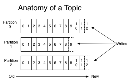
For each topic, the Kafka cluster maintains a partitioned log that looks like this:
Each partition is an ordered, immutable sequence of records that is continually appended to—a structured commit log. The records in the partitions are each assigned a sequential id number called the offset that uniquely identifies each record within the partition.
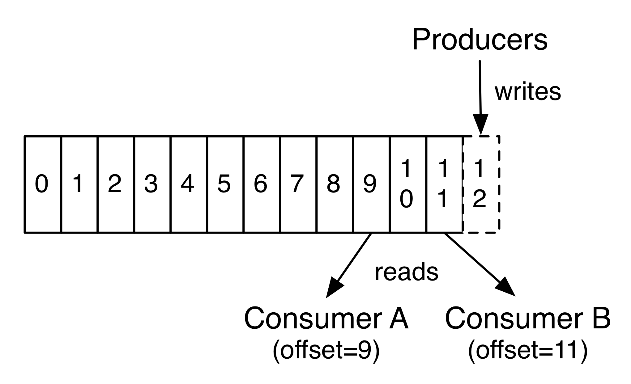
The Kafka cluster retains all published records—whether or not they have been consumed—using a configurable retention period. For example, if the retention policy is set to two days, then for the two days after a record is published, it is available for consumption, after which it will be discarded to free up space. Kafka's performance is effectively constant with respect to data size so storing data for a long time is not a problem.
In fact, the only metadata retained on a per-consumer basis is the offset or position of that consumer in the log. This offset is controlled by the consumer: normally a consumer will advance its offset linearly as it reads records, but, in fact, since the position is controlled by the consumer it can consume records in any order it likes. For example a consumer can reset to an older offset to reprocess data from the past or skip ahead to the most recent record and start consuming from "now".
This combination of features means that Kafka consumers are very cheap—they can come and go without much impact on the cluster or on other consumers. For example, you can use our command line tools to "tail" the contents of any topic without changing what is consumed by any existing consumers.
The partitions in the log serve several purposes. First, they allow the log to scale beyond a size that will fit on a single server. Each individual partition must fit on the servers that host it, but a topic may have many partitions so it can handle an arbitrary amount of data. Second they act as the unit of parallelism—more on that in a bit.

Distribution

The partitions of the log are distributed over the servers in the Kafka cluster with each server handling data and requests for a share of the partitions. Each partition is replicated across a configurable number of servers for fault tolerance.
Each partition has one server which acts as the "leader" and zero or more servers which act as "followers". The leader handles all read and write requests for the partition while the followers passively replicate the leader. If the leader fails, one of the followers will automatically become the new leader. Each server acts as a leader for some of its partitions and a follower for others so load is well balanced within the cluster.

Producers

Producers publish data to the topics of their choice. The producer is responsible for choosing which record to assign to which partition within the topic. This can be done in a round-robin fashion simply to balance load or it can be done according to some semantic partition function (say based on some key in the record). More on the use of partitioning in a second!

Consumers

Consumers label themselves with a consumer group name, and each record published to a topic is delivered to one consumer instance within each subscribing consumer group. Consumer instances can be in separate processes or on separate machines.
If all the consumer instances have the same consumer group, then the records will effectively be load balanced over the consumer instances.
If all the consumer instances have different consumer groups, then each record will be broadcast to all the consumer processes.
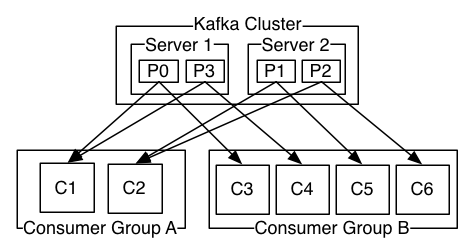
A two server Kafka cluster hosting four partitions (P0-P3) with two consumer groups. Consumer group A has two consumer instances and group B has four.
More commonly, however, we have found that topics have a small number of consumer groups, one for each "logical subscriber". Each group is composed of many consumer instances for scalability and fault tolerance. This is nothing more than publish-subscribe semantics where the subscriber is a cluster of consumers instead of a single process.
The way consumption is implemented in Kafka is by dividing up the partitions in the log over the consumer instances so that each instance is the exclusive consumer of a "fair share" of partitions at any point in time. This process of maintaining membership in the group is handled by the Kafka protocol dynamically. If new instances join the group they will take over some partitions from other members of the group; if an instance dies, its partitions will be distributed to the remaining instances.
Kafka only provides a total order over records within a partition, not between different partitions in a topic. Per-partition ordering combined with the ability to partition data by key is sufficient for most applications. However, if you require a total order over records this can be achieved with a topic that has only one partition, though this will mean only one consumer process per consumer group.

Guarantees

At a high-level Kafka gives the following guarantees:

• Messages sent by a producer to a particular topic partition will be appended in the order they are sent. That is, if a record M1 is sent by the same producer as a record M2, and M1 is sent first, then M1 will have a lower offset than M2 and appear earlier in the log.
• A consumer instance sees records in the order they are stored in the log.
• For a topic with replication factor N, we will tolerate up to N-1 server failures without losing any records committed to the log.

More details on these guarantees are given in the design section of the documentation.

Kafka as a Messaging System

How does Kafka's notion of streams compare to a traditional enterprise messaging system?
Messaging traditionally has two models: queuing and publish-subscribe. In a queue, a pool of consumers may read from a server and each record goes to one of them; in publish-subscribe the record is broadcast to all consumers. Each of these two models has a strength and a weakness. The strength of queuing is that it allows you to divide up the processing of data over multiple consumer instances, which lets you scale your processing. Unfortunately, queues aren't multi-subscriber—once one process reads the data it's gone. Publish-subscribe allows you broadcast data to multiple processes, but has no way of scaling processing since every message goes to every subscriber.
The consumer group concept in Kafka generalizes these two concepts. As with a queue the consumer group allows you to divide up processing over a collection of processes (the members of the consumer group). As with publish-subscribe, Kafka allows you to broadcast messages to multiple consumer groups.
The advantage of Kafka's model is that every topic has both these properties—it can scale processing and is also multi-subscriber—there is no need to choose one or the other.
Kafka has stronger ordering guarantees than a traditional messaging system, too.
A traditional queue retains records in-order on the server, and if multiple consumers consume from the queue then the server hands out records in the order they are stored. However, although the server hands out records in order, the records are delivered asynchronously to consumers, so they may arrive out of order on different consumers. This effectively means the ordering of the records is lost in the presence of parallel consumption. Messaging systems often work around this by having a notion of "exclusive consumer" that allows only one process to consume from a queue, but of course this means that there is no parallelism in processing.
Kafka does it better. By having a notion of parallelism—the partition—within the topics, Kafka is able to provide both ordering guarantees and load balancing over a pool of consumer processes. This is achieved by assigning the partitions in the topic to the consumers in the consumer group so that each partition is consumed by exactly one consumer in the group. By doing this we ensure that the consumer is the only reader of that partition and consumes the data in order. Since there are many partitions this still balances the load over many consumer instances. Note however that there cannot be more consumer instances in a consumer group than partitions.

Kafka as a Storage System

Any message queue that allows publishing messages decoupled from consuming them is effectively acting as a storage system for the in-flight messages. What is different about Kafka is that it is a very good storage system.
Data written to Kafka is written to disk and replicated for fault-tolerance. Kafka allows producers to wait on acknowledgement so that a write isn't considered complete until it is fully replicated and guaranteed to persist even if the server written to fails.
The disk structures Kafka uses scale well—Kafka will perform the same whether you have 50 KB or 50 TB of persistent data on the server.
As a result of taking storage seriously and allowing the clients to control their read position, you can think of Kafka as a kind of special purpose distributed filesystem dedicated to high-performance, low-latency commit log storage, replication, and propagation.

Kafka for Stream Processing

It isn't enough to just read, write, and store streams of data, the purpose is to enable real-time processing of streams.
In Kafka a stream processor is anything that takes continual streams of data from input topics, performs some processing on this input, and produces continual streams of data to output topics.
For example, a retail application might take in input streams of sales and shipments, and output a stream of reorders and price adjustments computed off this data.
It is possible to do simple processing directly using the producer and consumer APIs. However for more complex transformations Kafka provides a fully integrated Streams API. This allows building applications that do non-trivial processing that compute aggregations off of streams or join streams together.
This facility helps solve the hard problems this type of application faces: handling out-of-order data, reprocessing input as code changes, performing stateful computations, etc.
The streams API builds on the core primitives Kafka provides: it uses the producer and consumer APIs for input, uses Kafka for stateful storage, and uses the same group mechanism for fault tolerance among the stream processor instances.

Putting the Pieces Together

This combination of messaging, storage, and stream processing may seem unusual but it is essential to Kafka's role as a streaming platform.
A distributed file system like HDFS allows storing static files for batch processing. Effectively a system like this allows storing and processing historical data from the past.
A traditional enterprise messaging system allows processing future messages that will arrive after you subscribe. Applications built in this way process future data as it arrives.
Kafka combines both of these capabilities, and the combination is critical both for Kafka usage as a platform for streaming applications as well as for streaming data pipelines.
By combining storage and low-latency subscriptions, streaming applications can treat both past and future data the same way. That is a single application can process historical, stored data but rather than ending when it reaches the last record it can keep processing as future data arrives. This is a generalized notion of stream processing that subsumes batch processing as well as message-driven applications.
Likewise for streaming data pipelines the combination of subscription to real-time events make it possible to use Kafka for very low-latency pipelines; but the ability to store data reliably make it possible to use it for critical data where the delivery of data must be guaranteed or for integration with offline systems that load data only periodically or may go down for extended periods of time for maintenance. The stream processing facilities make it possible to transform data as it arrives.
For more information on the guarantees, apis, and capabilities Kafka provides see the rest of the documentation.

My next blog is about how we use Kafka using python.
Subscribe my blog for further interesting blogs

Read More

Flask Python API library

Eager to get started? This page gives a good introduction to Flask. It assumes you already have Flask installed.

Requirements

If you have a computer that runs Python then you are probably good to go. The tutorial application should run just fine on  Linux. Unless noted, the code presented in these articles has been tested against Python 2.7 and 3.4, though it will likely be okay if you use a newer 3.x release.

You should use pip to install and deploy Flask. To install Flask generally on your system, give this command on the command prompt:

       pip install flask

Note that you can also specify the Flask version, should you need (you won't need this one):

       pip install flask=0.10

This should install Flask and everything it depends on. Don't be surprised if you find it has installed several Python modules as a result.

Flask should now be installed! Now, time to create our first app.

A Minimal Application

A minimal Flask application looks something like this:

from flask import Flask
app = Flask(__name__)

@app.route('/')
def hello_world():
    return 'Hello, World!'

So what did that code do?

1. First we imported the Flask class. An instance of this class will be our WSGI application.
2. Next we create an instance of this class. The first argument is the name of the application’s module or package. If you are using a single module (as in this example), you should use __name__ because depending on if it’s started as application or imported as module the name will be different ('__main__' versus the actual import name). This is needed so that Flask knows where to look for templates, static files, and so on. For more information have a look at the Flask documentation.
3. We then use the route() decorator to tell Flask what URL should trigger our function.
4. The function is given a name which is also used to generate URLs for that particular function, and returns the message we want to display in the user’s browser.

Just save it as hello.py or something similar. Make sure to not call your application flask.py because this would conflict with Flask itself.
To run the application you can either use the flask command or python’s -m switch with Flask. Before you can do that you need to tell your terminal the application to work with by exporting the FLASK_APP environment variable:

$ export FLASK_APP=hello.py
$ flask run
 * Running on http://127.0.0.1:5000/

If you are on Windows you need to use set instead of export.
Alternatively you can use python -m flask:

$ export FLASK_APP=hello.py
$ python -m flask run
 * Running on http://127.0.0.1:5000/

This launches a very simple builtin server, which is good enough for testing but probably not what you want to use in production.
Now head over to http://127.0.0.1:5000/, and you should see your hello world greeting.

Externally Visible Server

If you run the server you will notice that the server is only accessible from your own computer, not from any other in the network. This is the default because in debugging mode a user of the application can execute arbitrary Python code on your computer.
If you have the debugger disabled or trust the users on your network, you can make the server publicly available simply by adding --host=0.0.0.0 to the command line:

flask run --host=0.0.0.0

This tells your operating system to listen on all public IPs.

What to do if the Server does not Start

In case the python -m flask fails or flask does not exist, there are multiple reasons this might be the case. First of all you need to look at the error message.

Old Version of Flask

Versions of Flask older than 0.11 use to have different ways to start the application. In short, the flask command did not exist, and neither did python -m flask.

Invalid Import Name

The FLASK_APP environment variable is the name of the module to import at flask run. In case that module is incorrectly named you will get an import error upon start (or if debug is enabled when you navigate to the application). It will tell you what it tried to import and why it failed.
The most common reason is a typo or because you did not actually create an app object.

Debug Mode

(Want to just log errors and stack traces? )
The flask script is nice to start a local development server, but you would have to restart it manually after each change to your code. That is not very nice and Flask can do better. If you enable debug support the server will reload itself on code changes, and it will also provide you with a helpful debugger if things go wrong.
To enable debug mode you can export the FLASK_DEBUG environment variable before running the server:

$ export FLASK_DEBUG=1
$ flask run

(On Windows you need to use set instead of export).
This does the following things:

1. it activates the debugger
2. it activates the automatic reloader
3. it enables the debug mode on the Flask application.

Attention

Even though the interactive debugger does not work in forking environments (which makes it nearly impossible to use on production servers), it still allows the execution of arbitrary code. This makes it a major security risk and therefore it must never be used on production machines.

Read More

GDB and it's use

What is GDB?

GDB, the GNU Project debugger, allows you to see what is going on `inside' another program while it executes -- or what another program was doing at the moment it crashed.
GDB can do four main kinds of things (plus other things in support of these) to help you catch bugs in the act:

• Start your program, specifying anything that might affect its behavior.
• Make your program stop on specified conditions.
• Examine what has happened, when your program has stopped.
• Change things in your program, so you can experiment with correcting the effects of one bug and go on to learn about another.

The program being debugged can be written in Ada, C, C++, Objective-C, Pascal (and many other languages). Those programs might be executing on the same machine as GDB (native) or on another machine (remote). GDB can run on most popular UNIX and Microsoft Windows variants.

GDB is a well known debugger library for  c and c++.  GDB is usually use for large and distributed system debugging. GDB is command line tool and has almost all function that you use in debugging using IDE.
I have explain some basic and useful methods of GDB that help up in learning GDB and debugging your programs
Installation

Before you go for installation first check either GDB is already installed or not. You check using this command
gd -help

I GDB is already installed on your machine, it shows all the available options of GDB.
If not installed it show message to install GDB.  Then you install it manually but first check these prerequisites

• An ANSI-compliant C compiler (gcc is recommended - note that gdb can debug codes generated by other compilers)
• 115 MB of free disk space is required on the partition on which you're going to build gdb.
• 
  
• 20 MB of free disk space is required on the partition on which you're going to install gdb.

Now run this command to install GDB

sudo apt-get install gdb

 GDB Command Line Arguments:

Starting GDB:

• gdb name-of-executable
• gdb -e name-of-executable -c name-of-core-file
• gdb name-of-executable --pid=process-id
  Use ps -auxw to list process id's: Attach to a process already running:
  

  [prompt]$ ps -auxw | grep myapp
  user1     2812  0.7  2.0 1009328 164768 ?      Sl   Jun07   1:18 /opt/bin/myapp
  [prompt]$ gdb /opt/bin/myapp 2812
  OR
  [prompt]$ gdb /opt/bin/myapp --pid=2812
              

Command line options: (version 6. Older versions use a single "-")

Option	Description
--help -h	List command line arguments
--exec=file-name -e file-name	Identify executable associated with core file.
--core=name-of-core-file -c name-of-core-file	Specify core file.
--command=command-file -x command-file	File listing GDB commands to perform. Good for automating set-up.
--directory=directory -d directory	Add directory to the path to search for source files.
--cd=directory	Run GDB using specified directory as the current working directory.
--nx -n	Do not execute commands from ~/.gdbinit initialization file. Default is to look at this file and execute the list of commands.
--batch -x command-file	Run in batch (not interactive) mode. Execute commands from file. Requires -x option.
--symbols=file-name -s file-name	Read symbol table from file file.
--se=file-name	Use FILE as symbol file and executable file.
--write	Enable writing into executable and core files.
--quiet -q	Do not print the introductory and copyright messages.
--tty=device	Specify device for running program's standard input and output.
--tui	Use a terminal user interface. Console curses based GUI interface for GDB. Generates a source and debug console area.
--pid=process-id -p process-id	Specify process ID number to attach to.
--version	Print version information and then exit.

GDB Commands:

Commands used within GDB:

Command	Description
help	List gdb command topics.
help topic-classes	List gdb command within class.
help command	Command description. eg help show to list the show commands
apropos search-word	Search for commands and command topics containing search-word.
info args i args	List program command line arguments
info breakpoints	List breakpoints
info break	List breakpoint numbers.
info break breakpoint-number	List info about specific breakpoint.
info watchpoints	List breakpoints
info registers	List registers in use
info threads	List threads in use
info set	List set-able option
Break and Watch
break funtion-name break line-number break ClassName::functionName	Suspend program at specified function of line number.
break +offset break -offset	Set a breakpoint specified number of lines forward or back from the position at which execution stopped.
break filename:function	Don't specify path, just the file name and function name.
break filename:line-number	Don't specify path, just the file name and line number. break Directory/Path/filename.cpp:62
break *address	Suspend processing at an instruction address. Used when you do not have source.
break line-number if condition	Where condition is an expression. i.e. x > 5 Suspend when boolean expression is true.
break line thread thread-number	Break in thread at specified line number. Use info threads to display thread numbers.
tbreak	Temporary break. Break once only. Break is then removed. See "break" above for options.
watch condition	Suspend processing when condition is met. i.e. x > 5
clear clear function clear line-number	Delete breakpoints as identified by command option. Delete all breakpoints in function Delete breakpoints at a given line
delete d	Delete all breakpoints, watchpoints, or catchpoints.
delete breakpoint-number delete range	Delete the breakpoints, watchpoints, or catchpoints of the breakpoint ranges specified as arguments.
disable breakpoint-number-or-range enable breakpoint-number-or-range	Does not delete breakpoints. Just enables/disables them. Example: Show breakpoints: info break Disable: disable 2-9
enable breakpoint-number once	Enables once
continue c	Continue executing until next break point/watchpoint.
continue number	Continue but ignore current breakpoint number times. Usefull for breakpoints within a loop.
finish	Continue to end of function.
Line Execution
step s step number-of-steps-to-perform	Step to next line of code. Will step into a function.
next n next number	Execute next line of code. Will not enter functions.
until until line-number	Continue processing until you reach a specified line number. Also: function name, address, filename:function or filename:line-number.
info signals info handle handle SIGNAL-NAME option	Perform the following option when signal recieved: nostop, stop, print, noprint, pass/noignore or nopass/ignore
where	Shows current line number and which function you are in.
Stack
backtrace bt bt inner-function-nesting-depth bt -outer-function-nesting-depth	Show trace of where you are currently. Which functions you are in. Prints stack backtrace.
backtrace full	Print values of local variables.
frame frame number f number	Show current stack frame (function where you are stopped) Select frame number. (can also user up/down to navigate frames)
up down up number down number	Move up a single frame (element in the call stack) Move down a single frame Move up/down the specified number of frames in the stack.
info frame	List address, language, address of arguments/local variables and which registers were saved in frame.
info args info locals info catch	Info arguments of selected frame, local variables and exception handlers.
Source Code
list l list line-number list function list - list start#,end# list filename:function	List source code.
set listsize count show listsize	Number of lines listed when list command given.
directory directory-name dir directory-name show directories	Add specified directory to front of source code path.
directory	Clear sourcepath when nothing specified.
Machine Language
info line info line number	Displays the start and end position in object code for the current line in source. Display position in object code for a specified line in source.
disassemble 0xstart 0xend	Displays machine code for positions in object code specified (can use start and end hex memory values given by the info line command.
stepi si nexti ni	step/next assembly/processor instruction.
x 0xaddress x/nfu 0xaddress	Examine the contents of memory. Examine the contents of memory and specify formatting. n: number of display items to print f: specify the format for the output u: specify the size of the data unit (eg. byte, word, ...) Example: x/4dw var
Examine Variables
print variable-name p variable-name p file-name::variable-name p 'file-name'::variable-name	Print value stored in variable.
p *array-variable@length	Print first # values of array specified by length. Good for pointers to dynamicaly allocated memory.
p/x variable	Print as integer variable in hex.
p/d variable	Print variable as a signed integer.
p/u variable	Print variable as a un-signed integer.
p/o variable	Print variable as a octal.
p/t variable x/b address x/b &variable	Print as integer value in binary. (1 byte/8bits)
p/c variable	Print integer as character.
p/f variable	Print variable as floating point number.
p/a variable	Print as a hex address.
x/w address x/4b &variable	Print binary representation of 4 bytes (1 32 bit word) of memory pointed to by address.
ptype variable ptype data-type	Prints type definition of the variable or declared variable type. Helpful for viewing class or struct definitions while debugging.
GDB Modes
set gdb-option value	Set a GDB option
set logging on set logging off show logging set logging file log-file	Turn on/off logging. Default name of file is gdb.txt
set print array on set print array off show print array	Default is off. Convient readable format for arrays turned on/off.
set print array-indexes on set print array-indexes off show print array-indexes	Default off. Print index of array elements.
set print pretty on set print pretty off show print pretty	Format printing of C structures.
set print union on set print union off show print union	Default is on. Print C unions.
set print demangle on set print demangle off show print demangle	Default on. Controls printing of C++ names.
Start and Stop
run r run command-line-arguments run < infile > outfile	Start program execution from the beginning of the program. The command break main will get you started. Also allows basic I/O redirection.
continue c	Continue execution to next break point.
kill	Stop program execution.
quit q	Exit GDB debugger.

 GDB Operation:

• Compile with the "-g" option (for most GNU and Intel compilers) which generates added information in the object code so the debugger can match a line of source code with the step of execution.
• Do not use compiler optimization directive such as "-O" or "-O2" which rearrange computing operations to gain speed as this reordering will not match the order of execution in the source code and it may be impossible to follow.
• control+c: Stop execution. It can stop program anywhere, in your source or a C library or anywhere.
• To execute a shell command: ! command
  or shell command
• GDB command completion: Use TAB key
  info bre + TAB will complete the command resulting in info breakpoints
  Press TAB twice to see all available options if more than one option is available or type "M-?" + RETURN.
• GDB command abreviation:
  info bre + RETURN will work as bre is a valid abreviation for breakpoints

Read More